Support Vector Machines for Classification on SET100 Returns

Note

The project was the CQF exam in Machine Learning in Finance.

Problem Understanding

The SET100 index, representing the top 100 stocks on the Stock Exchange of Thailand (SET), serves as a critical benchmark for Thailand’s equity market. Unlike established indices in developed markets such as the S&P 500 or the FTSE 100, the SET100 is exposed to the dynamic economic landscape of an emerging market. Emerging markets like Thailand offer higher growth potential due to industrialization, urbanization, and favorable demographics. However, this growth comes with increased volatility and higher risks, influenced by political instability, economic fluctuations, and global economic shocks.

The SET100 provides unique investment opportunities across diverse sectors, including finance, energy, consumer goods, and industrials. The inclusion of small to medium-sized enterprises in the index underscores its potential for significant growth. These features, along with the challenges and opportunities inherent in emerging markets, make the SET100 an intriguing subject for financial analysis and return prediction.

Accurately predicting stock returns is crucial for informed investment decisions. The volatile and complex nature of financial markets, with factors like market sentiment, economic indicators, and geopolitical events, poses significant challenges for return prediction. Traditional statistical methods often fail to capture the non-linear relationships within the data, necessitating more advanced machine learning techniques. In this project, we employ Support Vector Machines (SVM) to classify the daily returns of SET100 stocks, leveraging the algorithm’s capability to handle high-dimensional data and model complex patterns. Our goal is to enhance predictive accuracy, providing valuable insights for investors and portfolio managers.

Data Retrieving

The data for this study, including the open, high, low, and close (OHLC) prices of the SET100 stocks, was retrieved from Investing.com. The dataset spans from January 3, 2018, to May 30, 2024, providing a comprehensive range of historical price data here. All prices are adjusted for dividends and are presented in Thai Baht (THB). Upon retrieval, the data underwent a thorough cleaning process to ensure its quality and reliability. This process involved handling missing values, removing any duplicates, and ensuring consistency in the date formats.

Data Visualization/Description

The dataset includes the following primary features:

• Open: The opening price of the stock on a given trading day.
• High: The highest price of the stock during the trading day.
• Low: The lowest price of the stock during the trading day.
• Close: The closing price of the stock on the trading day.

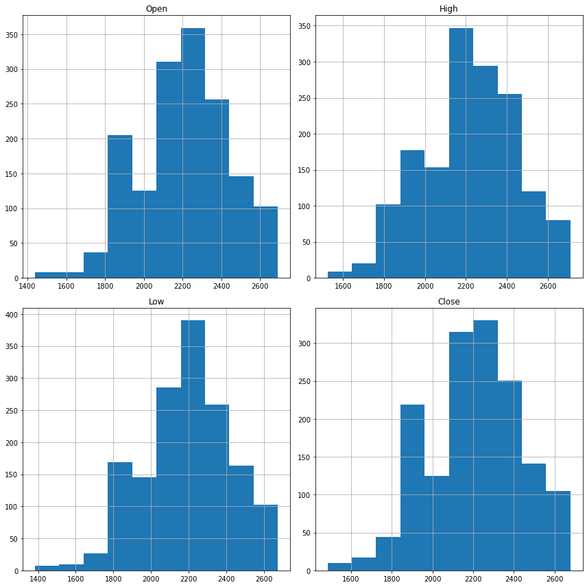
Figure 1 displays the distributions of some selected features, providing insights into their ranges and central tendencies. There are no extreme outliers in the data. Since the SET100 does not grow rapidly compared to other markets and the investigation period is relatively short, the histograms of the features show central tendencies. Additionally, these features are highly correlated. Feature engineering is necessary to capture the underlying patterns and improve the model’s performance.

Data Cleansing/Wrangling

Effective data cleansing and wrangling are crucial steps in preparing the dataset for analysis and modeling. In this study, the dataset consisting of the SET100 index’s historical price data underwent a thorough data cleansing process to ensure its quality and reliability.

Handling Missing Values

Missing values in the dataset can lead to inaccurate results and bias in the model. To address this, we performed the following steps:

• Identified missing values in the dataset.
• Imputed missing values using forward fill or backward fill methods, where appropriate.
• For features where imputation was not suitable, rows with missing values were removed to maintain data integrity.

Removing Duplicates

Duplicate records can distort the analysis and lead to incorrect conclusions. We ensured the dataset was free from duplicates by:

• Identifying and removing any duplicate rows based on the ‘Date’ column.

In this process, 70% of the data was allocated to the training set, and 30% to the testing set. The \texttt{random_state} parameter was set to 42 to ensure reproducibility of the results.

Feature Engineering

The following table lists the transformed features, their descriptions, and the mathematical formulas used to calculate them:

Feature	Description	Mathematical Formula
Volatility	Standard deviation of returns over a rolling window of 10 days. It captures the degree of variation in stock prices, indicating market uncertainty and risk.	$\text{std}(\text{Return}_{t-10:t-1})$
Momentum	Difference between the current close price and the close price 10 days ago. This feature helps identify the trend and strength of stock price movements.	$\text{Close}_{t-10} - \text{Close}_{t-20}$
Avg_Open_Close	Average of the open and close prices. It provides a smoothed value representing the central tendency of the prices within a trading day.	$\frac{\text{Open}_{t-1} + \text{Close}_{t-1}}{2}$
Avg_High_Low	Average of the high and low prices, gives an insight into the range of price fluctuations within a day, indicating the volatility within a single trading day.	$\frac{\text{High}_{t-1} + \text{Low}_{t-1}}{2}$
Price_Range	Difference between the high and low prices, this feature shows the price movement within a day.	$\text{High}_{t-1} - \text{Low}_{t-1}$
Daily_Change	Difference between the close and open prices.	$\text{Close}_{t-1} - \text{Open}_{t-1}$
Daily_Change_Percent	Daily change as a percentage of the open price, offering a normalized view of daily price changes.	$\frac{\text{Daily_Change}_{t}}{\text{Open}_{t-1}} \times 100$
Rolling_Mean_Close	Rolling mean of the close prices over a 10-day window, provides a smoothed trend of the closing prices.	$\text{mean}(\text{Close}_{t-10:t-1})$
Rolling_Mean_Volume	Rolling mean of volatility over a 10-day window, highlighting longer-term trends in market volatility.	$\text{mean}(\text{Volatility}_{t-10:t-1})$
Rolling_Mean_Momentum	Rolling mean of momentum over a 10-day window, helps in identifying sustained trends in price movements.	$\text{mean}(\text{Momentum}_{t-10:t-1})$

By engineering these features, we transformed raw stock price data into a structured dataset that captures essential financial metrics, facilitating effective modeling and prediction using the SVM approach.

Data Modelling

Support Vector Machine

SVM works by finding the hyperplane that best separates the classes in the feature space. The hyperplane is chosen to maximize the margin, which is the distance between the hyperplane and the nearest data points from each class.

For a linear SVM, the decision function is defined as:

$$ f(\mathbf{x}) = \mathbf{w} \cdot \mathbf{x} + b $$

where $\mathbf{w}$ is the weight vector, $\mathbf{x}$ is the input vector, and $b$ is the bias term. The hyperplane is defined by the equation $\mathbf{w} \cdot \mathbf{x} + b = 0$.

The objective of SVM is to maximize the margin while correctly classifying the training data. This can be formulated as a constrained optimization problem:

$$ \min_{\mathbf{w}, b} \frac{1}{2} \|\mathbf{w}\|^2 + C \sum_{i=1}^{n} \xi_i $$ $$ \text{subject to } y_i (\mathbf{w} \cdot \mathbf{x}_i + b) \geq 1 \quad \forall i $$

where $y_i$ are the class labels, and $\mathbf{x}_i$ are the input vectors, $\xi_i \geq 0 \quad \forall i$, and $C$ is the regularization parameter.

A larger value of $C$ puts more emphasis on minimizing the misclassification errors, potentially at the expense of a smaller margin. This can lead to a model that fits the training data very closely (low bias but high variance), which may result in overfitting.

Conversely, a smaller value of $C$ puts more emphasis on maximizing the margin, allowing some misclassifications. This can lead to a simpler model that may generalize better to unseen data (high bias but low variance), reducing the risk of overfitting.

This project employs the kernal trick with linear, RBF, and Sigmoid kernels as can be found in the Appendix \ref{app:A}.

Model Selection via Parameter Optimization

To optimize the performance of the SVM model, we employed Grid Search, a systematic approach to hyperparameter tuning. Grid Search involves evaluating a model’s performance across a predefined set of hyperparameters to identify the combination that yields the best results.

In this study, we considered three key hyperparameters for the SVM model:

• $C$: The regularization parameter, which controls the trade-off between achieving a low error on the training data and minimizing the model complexity to avoid overfitting.
• $\gamma$: The kernel coefficient for non-linear kernels (e.g., Radial Basis Function, RBF). It defines how far the influence of a single training example reaches, with low values meaning ‘far’ and high values meaning ‘close’.
• kernel: The type of kernel function used to transform the input data. We considered two kernel types: Linear and Radial Basis Function, and Sigmiod Kernels.

We defined a grid of hyperparameters with the following values $C \in \{0.1, 1, 10, 100\}$, $\gamma \in \{1, 0.1, 0.01, 0.001\}$, and three types of kernel as discuses previous. The grid defined above results in a total of 48 combinations (4 values for $C$, 4 values for $\gamma$, and 3 values for kernel). Each combination was evaluated to determine the optimal set of hyperparameters. After performing the Grid Search, the best parameters were found to be: $C = 1$ in the linear kernel.

In practice, Python’s scikit-learn library uses the Sequential Minimal Optimization (SMO) algorithm [2] to solve the dual formulation of the SVM optimization problem [1]. SMO breaks the problem into smaller sub-problems, each involving only two Lagrange multipliers at a time, which makes the optimization more efficient and scalable. The details can be explored in Appendix \ref{app:smo}.

Model Validation/Evolution

The model performance is listed in Table \ref{tab:classification_report}. The SVM model achieved an accuracy of 65.80%, indicating a high rate of correct predictions. The precision for class 0.0 (negative returns) was 0.68, and for class 1.0 (positive returns) it was 0.62, demonstrating the model’s ability to correctly identify negative returns more accurately than positive returns. The recall for class 0.0 was 0.74, and for class 1.0 it was 0.55, indicating that the model successfully identified a majority of actual negative returns but less so for positive returns. The F1-scores for both classes were moderate (0.71 for class 0.0 and 0.58 for class 1.0), reflecting a balance between precision and recall. The ROC AUC score of 0.64 further validates the model’s discriminatory ability between positive and negative returns.

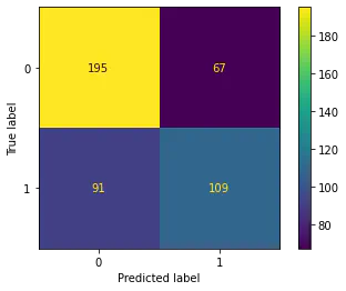
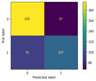
The confusion matrix, shown in Figure 2, provided detailed insights into the model’s predictions. Out of 462 total predictions, the model made a balanced number of correct and incorrect predictions for both classes. Specifically, it accurately predicted 194 true negatives and 110 true positives, underscoring its reliability in distinguishing between the two classes but also highlighting areas for improvement.

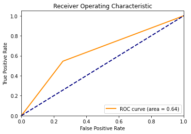
The ROC AUC score, which stands for Receiver Operating Characteristic Area Under Curve, shown in Figure 3, is a measure of the model’s ability to distinguish between classes. An ROC AUC score of 0.64 indicates a moderate level of distinction between positive and negative returns, suggesting that the model is better than random guessing but still has room for improvement.

Trading Implication

The moderate accuracy and performance metrics of the SVM model suggest potential applications in financial trading strategies. For instance, predictions of positive returns (Class 1.0) could serve as buy signals, whereas negative return predictions (Class 0.0) might indicate sell or hold actions. This predictive capability can be integrated into automated trading systems to enhance decision-making processes. Moreover, incorporating risk management strategies, such as setting stop-loss orders based on volatility predictions, can mitigate potential losses. Portfolio optimization can also benefit from these predictions by diversifying investments across multiple stocks within the SET100, thereby balancing risk and return.

Metric	Precision	Recall	F1-Score	Support
0	0.68	0.74	0.71	262
1	0.62	0.55	0.58	200
Accuracy	0.66	0.66	0.66	462
Macro Avg	0.65	0.64	0.65	462
Weighted Avg	0.65	0.66	0.65	462

Table: Classification Report and Metrics

Appendix

Kernel Trick

SVM can efficiently perform non-linear classification using kernel functions. Kernels transform the input data into a higher-dimensional space where a linear separator can be used to distinguish between classes. Here, we describe three commonly used kernels: Linear, Radial Basis Function (RBF), and Sigmoid.

Linear Kernel

The linear kernel is the simplest type of kernel, used when the data is linearly separable in the original feature space. The decision boundary is a hyperplane in the original feature space.

Mathematically, the linear kernel function is defined as:

$$ K(\mathbf{x}_i, \mathbf{x}_j) = \mathbf{x}_i \cdot \mathbf{x}_j $$

where $\mathbf{x}_i$ and $\mathbf{x}_j$ are input vectors, and $\cdot$ denotes the dot product.

The decision function for the linear kernel is given by:

$$ f(\mathbf{x}) = \mathbf{w} \cdot \mathbf{x} + b $$

where $\mathbf{w}$ is the weight vector and $b$ is the bias term.

Radial Basis Function (RBF) Kernel

The RBF kernel, also known as the Gaussian kernel, is a popular choice for SVMs because it can handle non-linear relationships by mapping the data into an infinite-dimensional space. It is particularly effective when the decision boundary is highly non-linear.

The RBF kernel function is defined as:

$$ K(\mathbf{x}_i, \mathbf{x}_j) = \exp\left(-\gamma \|\mathbf{x}_i - \mathbf{x}_j\|^2\right) $$

where $\gamma$ is a parameter that defines the width of the Gaussian function, and $\|\mathbf{x}_i - \mathbf{x}_j\|^2$ is the squared Euclidean distance between the input vectors.

The decision function for the RBF kernel is:

$$ f(\mathbf{x}) = \sum_{i=1}^{n} \alpha_i y_i \exp\left(-\gamma \|\mathbf{x} - \mathbf{x}_i\|^2\right) + b $$

where $\alpha_i$ are the Lagrange multipliers, $y_i$ are the class labels, and $b$ is the bias term.

Sigmoid Kernel

The sigmoid kernel is based on the sigmoid function, often used in neural networks. It can map the input data into a higher-dimensional space, similar to RBF, but is less commonly used.

The sigmoid kernel function is defined as:

$$ K(\mathbf{x}_i, \mathbf{x}_j) = \tanh\left(\gamma \mathbf{x}_i \cdot \mathbf{x}_j + c\right) $$

where $\alpha$and $c$ are kernel parameters, and $\tanh$ is the hyperbolic tangent function.

The decision function for the sigmoid kernel is:

$$ f(\mathbf{x}) = \tanh\left(\sum_{i=1}^{n} \gamma_i y_i (\mathbf{x} \cdot \mathbf{x}_i) + c\right) $$

where $\alpha_i$ are the Lagrange multipliers, $y_i$ are the class labels, and $c$ is a parameter.

SVM Dual Formulation

The optimization problem is often solved using its dual formulation. The dual problem focuses on finding the Lagrange multipliers $\alpha_i$ that satisfy the following:

$$ \max_{\alpha} \sum_{i=1}^{n} \alpha_i - \frac{1}{2} \sum_{i=1}^{n} \sum_{j=1}^{n} \alpha_i \alpha_j y_i y_j K(\mathbf{x}_i, \mathbf{x}_j) $$

subject to:

$$ 0 \leq \alpha_i \leq C \quad \forall i $$

and

$$ \sum_{i=1}^{n} \alpha_i y_i = 0 $$

where $K(\mathbf{x}_i, \mathbf{x}_j)$ is the kernel function that computes the dot product in the transformed feature space.

Sequential Minimal Optimization

The SMO algorithm works as follows:

• Initialize the Lagrange multipliers $\alpha_i$ to zero.
• item Repeat until convergence:
  1. Select two multipliers $\alpha_i$ and $\alpha_j$ that violate the Karush-Kuhn-Tucker (KKT) conditions.
  2. Solve the optimization problem for these two multipliers while keeping the others fixed.
  3. Update the multipliers and the corresponding weight vector $\mathbf{w}$ and bias term $b$.

The advantage of the SMO algorithm is that it decomposes the large quadratic programming problem into a series of smaller problems that are easier and faster to solve.

The optimization of two Lagrange multipliers $\alpha_i$ and $\alpha_j$ can be expressed as:

$$ \max_{\alpha_i, \alpha_j} \left( \alpha_i + \alpha_j - \frac{1}{2} \left( \alpha_i^2 K(\mathbf{x}_i, \mathbf{x}_i) + \alpha_j^2 K(\mathbf{x}_j, \mathbf{x}_j) + 2 \alpha_i \alpha_j K(\mathbf{x}_i, \mathbf{x}_j) \right) \right) $$

subject to the constraints:

$$ 0 \leq \alpha_i, \alpha_j \leq C $$

and

$$ y_i \alpha_i + y_j \alpha_j = \text{constant} $$

This quadratic optimization problem in two variables is much simpler to solve, and the SMO algorithm iteratively updates the multipliers to find the optimal solution.

References

[1] V. K. Chauhan, K. Dahiya, and A. Sharma. Problem formulations and solvers in linear svm: a review. Artificial Intelligence Review, 52(2):803–855, 2019.

[2] J. Platt. Sequential minimal optimization: A fast algorithm for training support vector machines. 1998.