Why the Lookback Option is More Expensive Than the Asian Option, A Simulation Approach

Note

The project was the CQF exam in Monte Carlo simulation for option pricing.

Introduction

Asian and lookback options, two distinct types of exotic options, differ fundamentally in their payoff structures, each designed to meet specific financial needs and risk profiles. Asian options, encompassing average price and average strike varieties, calculate their payoffs based on the average price of the underlying asset over a designated period. This averaging reduces the effects of volatility, often making these options less costly than standard options, which makes them particularly suitable for hedging in markets characterized by high volatility but indeterminate price trends.

In contrast, lookback options derive their payoffs from the highest or lowest price of the underlying asset during the life of the option. This feature ensures that the holder benefits from the most favorable price achieved during the option period, providing an optimal payoff scenario. Due to these characteristics, lookback options are generally more expensive than both standard and Asian options and are favored by investors anticipating significant market movements who aim to fully capitalize on these fluctuations.

In a complete market framework, the expected value of the discounted payoff under the risk-neutral probability measure $Q$ for any derivative’s price $V(S, t)$ can be mathematically formulated as:

$$ V(S, t) = e^{r(T-t)} \mathbb{E}^Q[\Lambda(S_T)] $$

where $r$ is the risk-free rate, $T$ is the time of expiry, $t$ is the current time, $S_T$ is the stock price at expiry, and $\Lambda(S_T)$ denotes the option’s specific payoff function.

Path-dependent options such as the arithmetic average-type call Asian option demonstrate the influence of the underlying asset’s historical prices on the payoff:

$$ \Lambda_{asian}(t) = (\bar{S} - K)^+, \ \text{where} \ \bar{S} = \frac{1}{m}\sum_{j = 1}^m S(t_j), $$

with $m$ representing the number of observation periods. Similarly, the fixed-strike lookback option’s payoff is determined by:

$$ \Lambda_{lookback}(t) = (S_{\text{max}} - K)^+ $$

where $S_{\text{max}}$ is the maximum price reached during the option’s duration. Both option payoffs can be readily found in the literature textbook such as the standard book by Hull and Basu [2].

While these options cannot be priced analytically within the traditional Black-Scholes framework, alternative analytical methods such as spectral theory have been employed to estimate the prices of Asian options [3]. However, this discussion will primarily focus on using the standard Euler-Maruyama scheme for approximating the prices of these options and explaination mathematically why the lockback option more expensive than the Asian option at the equivalent parameters in the subsequent section.

Numerical Method

The simplest approximation method for the log-normal price process is the Euler-Maruyama scheme, as discussed in [4], for simulating the stock price $S$ at time $t + \Delta t$ based on the stock price at time $t$. The formula is given by:

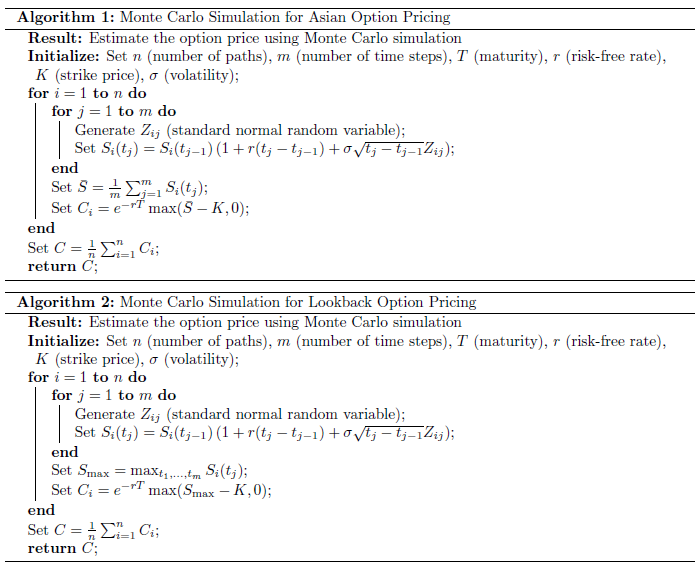
$$ S_i(t_j) = S_i(t_{j-1})\left(1 + r (t_j - t_{j-1}) + \sigma \sqrt{t_j - t_{j-1}} Z_{ij} \right) $$

where $r$ is the risk free rate, $S_i(t_j)$ is underlying asset price at the path index $i$ and time index $j$, $Z_{ij}$ is a standard normal variable . The algorithm for generating the path and estimating the expected discounted payoff is outlined in the following steps.

Simulation Results and Discussion

Following the discussed algorithms, we estimate the price of the Asian and lookback options by setting the parameters as the following list. Using the sample data provided:

• Initial stock price $S_0 = 100$
• Strike price $E = 100$
• Time to expiry $T-t = 1$ year
• Volatility $\sigma = 20\%$
• Constant risk-free interest rate $r = 5\%$

It is important to note that the standard Euler-Maruyama scheme is not efficient when applied to path-dependent options. A more effective discretization method that accounts for intermediate time effects was discussed in [1] on pages 7-8.

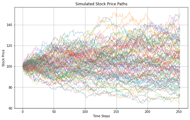
The 10,000 simple paths simulated are shown in Figure 1. The prices of the options follow a log-normal distribution. Next, the proposed algorithms are applied to estimate the prices of the options given the parameters. Here, the time step is set to $m = 252$ or one daily step.

• The price of the Asian option is 5.843582.
• The price of the lookback option is 18.348289.

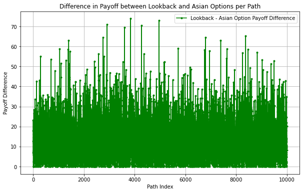
Figure 2 shows the difference in payoffs between lookback and Asian options for each path. The differences are all non-negative, implying that the payoff of the lookback option consistently dominates the Asian option payoff at equivalent parameters. This result is derived from their respective payoff functions. Since

$$ \max\{S(t_1), S(t_2), \dots, S(t_j)\} \geq \bar{S}(t), $$

it follows that:

$$ \Lambda_{asian}(t) \leq \Lambda_{lookback}(t). $$

It is straightforward to prove that the maximum function always dominates the average function, as discussed in the Appendix.

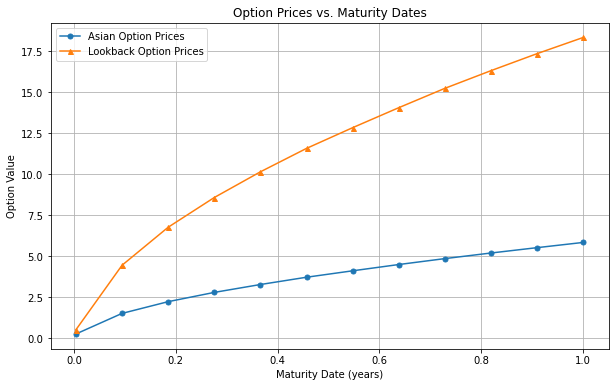
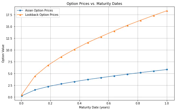
Next, it is crucial to consider what would happen to the spread of option prices if the maturity date varies. Figure 3 displays the difference between the lookback and Asian option prices at different maturities. As can be observed, the spread in price increases exponentially as the contract duration becomes longer. This makes sense because the issuer of the lookback option takes on more risk as the maximum value of the underlying price can be hit over a longer period. Conversely, the average payoff of the Asian option tends to be more predictable when the time series is extended, as a few samples will not significantly change the average of a large number.

Financially, lookback options effectively eliminate timing risk because the holder is guaranteed to benefit from the best prices achieved over the option’s life. This feature is particularly attractive in volatile markets, where predicting the optimal time to exercise an option can be challenging. Conversely, Asian options reduce the risk of market manipulation near expiration and mitigate the risk associated with short-term volatility. These characteristics make them less risky from the issuer’s perspective compared to lookback options.

Conclusion

This report has explored the financial characteristics and pricing mechanisms of call Asian and lookback options using the Euler-Maruyama simulation method. Our simulations confirm that lookback options consistently command higher prices than Asian options under equivalent parameters. This difference is attributed to the inherent payoff structures of the two options. Lookback options, which pay based on the maximum or minimum price reached by the underlying asset, provide a payoff that capitalizes on the optimal market conditions during the option’s life. Consequently, these options are particularly valuable in volatile markets where price peaks can be significant.

On the other hand, Asian options average the price of the underlying asset over a period, which tends to smooth out extremes of market movements. This characteristic not only reduces the cost of the option but also diminishes the payoff potential compared to lookback options. From a risk management perspective, Asian options offer a more stable but generally less lucrative investment compared to lookback options.

Appendix

Lemma: Let $X$ be the set of real numbers. Then,

$$ \bar{X} \leq \max X $$

Proof: Given that $\bar{X} = \frac{1}{m}\sum_{i = 1}^m x_i$, where $x_i \in X$, it follows that each $x_i \leq \max X$. Therefore, we have

$$ \bar{X} = \frac{1}{m}\sum_{i = 1}^m x_i \leq \frac{1}{m}\sum_{i = 1}^m \max X = \frac{1}{m} (m \max X) = \max X. $$

This shows that the average of the elements in \(X\) cannot exceed the maximum element in $X$.

References

[1] P. Glasserman. Monte Carlo methods in financial engineering volume 53. Springer, 2004.

[2] J. C. Hull and S. Basu. Options, futures, and other derivatives. Pearson Education India, 2016.

[3] V. Linetsky. Exact pricing of asian options: an application of spectral theory. Operat. Res, 2001.

[4] G. Maruyama. Continuous markov processes and stochastic equations. Rendiconti del Circolo Matematico di Palermo, 4:48–90, 1955.